 Siddharth
The Zipper, the Mask, and the Lost Write: How AI Picks the Right Numbers

Siddharth
October 17, 202636 min read
How AI works · A plain-English guide
A plain-English guide to one of the most common operations in machine learning — and the silent mistakes hiding in it.
By Siddharth Tiwari · AI strategy & analytics · 23 min read
Every time a streaming service suggests a film, a phone recognises its owner’s face, or a chatbot answers a question, a computer is doing something surprisingly humble: picking numbers out of grids. Underneath it all, modern AI is a vast collection of numbers in tables, and almost everything it does begins by pulling the right ones out. That act of picking is called indexing.
A tensor is a grid of numbers, like a spreadsheet: rows, columns and a number in every cell. Each direction you can move in, down the rows or across the columns, is called an axis (engineers also say dimension), and the tensor’s shape lists its size along each axis. Three rows and four columns make shape (3, 4).
Almost anything can become a tensor. A photo is a grid of tiny squares called pixels, each stored as a brightness number; a colour photo stacks three such grids, for red, green and blue. Sound is a long list of numbers. Text becomes numbers too: every word gets an ID and a row of numbers describing its meaning. An AI model is itself a giant stack of grids, often billions of numbers in all.
To index a tensor is to point at positions in it and take what is there: “row 2, column 3”, or “every cell above 100”. The position numbers are called indexes, and computers count them from 0, so the first row is row 0.
Picking is everywhere. A film recommender looks up the row of numbers that describes you and picks your best-scoring films. A translator swaps each word for its ID and picks that word’s row from a vocabulary table. Face recognition picks out the block of pixels holding a face, then the closest match among known faces. A chatbot writes one word at a time, scoring every possible next word and picking one. Indexing is one of the most common operations in AI code, and often the first thing a model does with your data.
Indexing follows precise rules, and some are surprising. Engineers who misread them rarely see an error message. They get answers that look right and are not: a model that learns from the wrong numbers, a correction that silently changes nothing, a step that copies gigabytes of data and burns costly time on GPUs, the specialised chips that run AI. Understanding these rules is understanding how AI handles information.
Each idea below comes in four layers: plain English with an everyday comparison, the precise rule, code for engineers, and why it matters. The code is optional.
Before the rules, a test of intuition. We will use a tiny tensor: twelve numbers in three rows of four, numbered 0 to 11 so that every cell is easy to find. The code is written in PyTorch, one of the most popular toolkits for building AI. In it, x is the grid; t is a second tensor made of two such grids, stacked like the pages of a book; and rmask and cmask are lists of yes/no answers (True or False). rmask says yes to rows 0 and 2, cmask says yes to columns 1 and 3, and lists like these are called masks. Square brackets after a name, as in x[...], are how code asks for cells.
>>> import torch
>>> x = torch.arange(12).reshape(3, 4)
>>> x
tensor([[ 0,  1,  2,  3],
        [ 4,  5,  6,  7],
        [ 8,  9, 10, 11]])
>>> t = torch.arange(24).reshape(2, 3, 4)            # two 3 x 4 layers
>>> rmask = torch.tensor([True, False, True])        # rows 0 and 2
>>> cmask = torch.tensor([False, True, False, True]) # columns 1 and 3
Predict before you read on
x[[0, 2], [1, 3]], meaning “rows 0 and 2, columns 1 and 3”. Most people expect four numbers: the corners 1, 3, 9 and 11.x[x % 3 == 0], meaning “every number divisible by 3”. Do they come back in their places in the grid?x[rmask][:, cmask] against x[rmask, cmask]: the same two masks, applied in two steps or in one. Same answer?x[rmask][:, cmask] = 0: set those cells to zero, in two steps. What happens to x?Here is what PyTorch 2.14 answers:
>>> x[[0, 2], [1, 3]]          # 1. not a 2 x 2 block
tensor([ 1, 11])
>>> x[x % 3 == 0]              # 2. not a 3 x 4 grid with holes
tensor([0, 3, 6, 9])
>>> x[rmask][:, cmask]         # 3. the chain builds a grid...
tensor([[ 1,  3],
        [ 9, 11]])
>>> x[rmask, cmask]            #    ...one bracket builds pairs
tensor([ 1, 11])
>>> x[rmask][:, cmask] = 0     # 4. no error...
>>> x                          #    ...and no change
tensor([[ 0,  1,  2,  3],
        [ 4,  5,  6,  7],
        [ 8,  9, 10, 11]])
In plain English: asking for two rows and two columns returned two numbers, not four. Asking for the multiples of three returned them in a flat line, with the grid gone. Doing the same selection in two steps or in one gave different answers. And the attempt to set cells to zero ran without complaint and changed nothing at all.
None of this is a bug. Every result follows from a handful of rules that PyTorch applies with complete consistency, nearly all of them inherited from NumPy, the library that set the conventions for numerical computing in Python. We will build those rules in eight stops, and by the end all four answers should look obvious. Every snippet on this page was run on PyTorch 2.14, and each one starts from the setup above.
In plain English
Think of the square brackets as a form with one box per axis. In x[1, 2:4], the first box holds 1 and talks about the rows; the second holds 2:4 and talks about the columns. We will call each box a slot. What goes in a slot decides what happens to that direction of the grid.
A single number, such as 1, means “row 1 only”, and the row direction disappears: we are left with one line of four numbers. A range, called a slice, such as 1:2 (“from row 1 up to, but not including, row 2”), means “this stretch of rows”, and the row direction survives, even when the stretch is a single row. It is the difference between tearing one line out of a spreadsheet and keeping a spreadsheet that happens to have one line. Two special markers complete the set: None adds a new direction of size 1, like slipping a single page into a folder, and ..., the ellipsis, means “every direction I have not mentioned”.
The precise rule
Walk the slots from left to right and build the output shape as you go:
..., consumes every axis the other slots do not name and passes them through unchanged.Any axes left over at the end behave as if we had written :, the slice that means “everything”, for them.
For engineers
>>> x[1]                    # integer: the row axis is gone
tensor([4, 5, 6, 7])
>>> x[1:2]                  # slice: the row axis survives with length 1
tensor([[4, 5, 6, 7]])
>>> x[None].shape           # None: a new leading axis
torch.Size([1, 3, 4])
>>> x[:, None].shape        # ...or a new axis between rows and columns
torch.Size([3, 1, 4])
>>> y = torch.arange(120).reshape(2, 3, 4, 5)
>>> y[0, ..., None].shape   # drop axis 0, keep (3, 4, 5), append 1
torch.Size([3, 4, 5, 1])
The difference between x[1] and x[1:2] is the first thing worth internalising. Both select the same four numbers, but one returns a vector of shape (4,) and the other a matrix of shape (1, 4). The data is identical; the contract is not. Integers are for when we are finished with an axis. Slices are for when that axis still means something downstream.
The edges of the rule are just as consistent. An integer must point at a position that exists, a slice is clamped to whatever exists, and a bracket cannot name more axes than the tensor has:
>>> x[5]
Traceback (most recent call last):
  ...
IndexError: index 5 is out of bounds for dimension 0 with size 3
>>> x[5:9].shape            # past the end: empty, not an error
torch.Size([0, 4])
>>> x[0, 0, 0]
Traceback (most recent call last):
  ...
IndexError: too many indices for tensor of dimension 2
Why it matters
Most shape mistakes in AI code are slot mistakes, and they rarely announce themselves. Writing a single number where later code expects a range, x[:, 0] instead of x[:, 0:1], silently changes how numbers line up a few lines further on. Ranges that run past the end are worse, because they never complain. A counting slip in the code that feeds a model its examples can produce an empty batch (the bundle of examples a model learns from at each step) instead of an error. The average of nothing is nan, “not a number”, and it flows quietly into the score the model is trying to improve.
In plain English
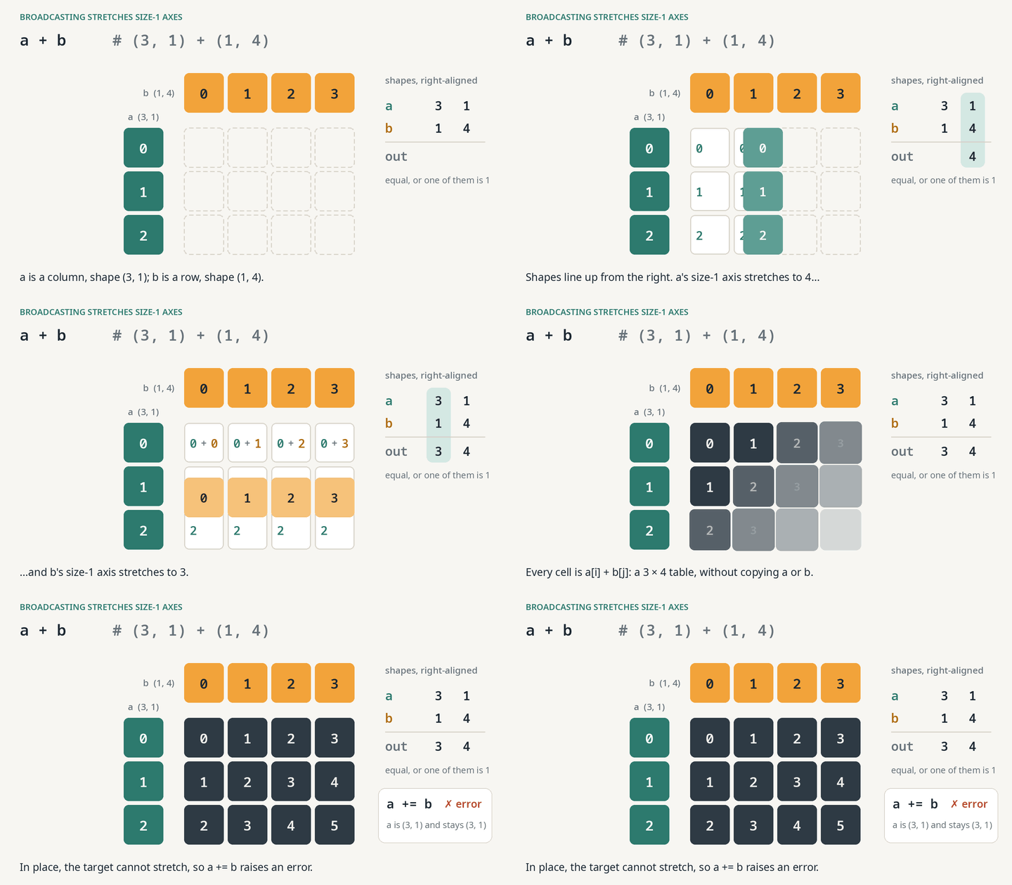
Suppose we want to add a column of three numbers to a row of four. They are different shapes, so PyTorch stretches each one until they fit: the column is repeated across four columns, the row is repeated down three rows, and every cell now holds one number from each. This stretching is called broadcasting. Picture laying the same one-row ruler across every row of a table. It only works when the pieces are compatible: in each direction the sizes must match, or one of them must be 1, so that it can stretch.
There is one catch. Ask PyTorch to put the answer back into the column itself, an in-place update that changes the original instead of making something new, and it refuses: the column has room for three numbers and the answer has twelve. Stretching works on the way in, never on the way back.
The precise rule
Write the two shapes one above the other, aligned on the right, and compare them column by column. The sizes must be equal, or one of them must be 1, in which case it stretches to match the other. A shape that runs out of axes on the left is padded with 1s. The result takes the larger size in every column.
In-place operations are one-way: the result must fit the target’s existing shape, because the target cannot grow.
For engineers
>>> a = torch.arange(3).reshape(3, 1)   # a column
>>> b = torch.arange(4).reshape(1, 4)   # a row
>>> a + b                               # (3, 1) + (1, 4) gives (3, 4)
tensor([[0, 1, 2, 3],
        [1, 2, 3, 4],
        [2, 3, 4, 5]])
>>> a += b                              # but a must stay (3, 1)
Traceback (most recent call last):
  ...
RuntimeError: output with shape [3, 1] doesn't match the broadcast shape [3, 4]
Nothing is copied to perform the stretch. PyTorch rereads the same values along the stretched axis (internally, with a stride of 0), so broadcasting a column across a million columns costs no extra memory for the input. The output is another matter: a + b really is a new 3 × 4 tensor.
Assignment follows the same one-way rule. The left-hand side fixes the shape, and the right-hand side must broadcast to it. That makes some writes pleasantly compact:
>>> x[[0, 2]] = torch.tensor([100, 200]).reshape(2, 1)  # fills (2, 4)
>>> x
tensor([[100, 100, 100, 100],
        [  4,   5,   6,   7],
[200, 200, 200, 200]])Why it matters
The dangerous stretches are the ones that succeed. Suppose a model produces its predictions as a column of N numbers while the correct answers sit in a flat list of N. Subtracting one from the other should give N differences. Broadcasting instead stretches them into an N × N table, comparing every prediction with every answer. Every entry is a real number, so training carries on, measuring the wrong thing, and nothing crashes. PyTorch’s ready-made error measure, F.mse_loss, warns about exactly this mismatch; hand-written code does not. When a shape matters, check it.
In plain English
When we ask for part of a tensor, PyTorch can answer in one of two ways. It can hand us a view: a window onto the original. No numbers move; we simply see a region of the same data, so changing a number through the window changes the original. Or it can hand us a copy: a photocopy of the numbers we asked for, on fresh memory, so writing on it never touches the original.
Which one we get depends on how we asked, not on what we asked for. Single numbers and ranges describe a regular pattern of positions, so they give a window. Lists of positions and masks can name any cells in any order, so they give a photocopy, even when they happen to pick a perfectly regular block. Engineers call the first kind basic indexing and the second advanced indexing.
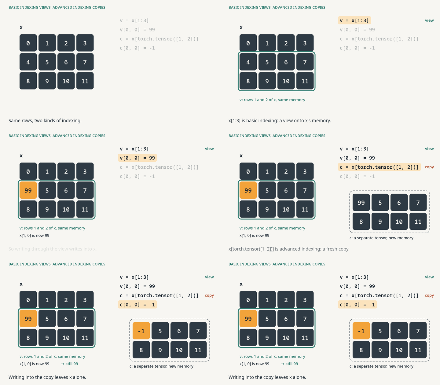
x, so writing 99 through it changes x. Asking with a list of positions gives a photocopy, so writing -1 on it leaves x alone.The precise rule
Ask one question of every bracket: could the result be described as a starting point plus a fixed step along each axis of the original (an offset and strides)? Integers, slices, None and the ellipsis always can, so they give views. Lists, integer tensors and masks name positions, so they give copies, even when those positions happen to form a tidy slice.
For engineers
The four slot types from stop 1 share a property: their result can always be described as a starting offset plus a stride per axis into the original memory. So PyTorch moves no data at all. It returns a view, a new tensor header that points into the same storage. Python lists, integer tensors and boolean masks name arbitrary positions, which in general cannot be expressed as strides, so PyTorch gathers the selected values into fresh memory and returns a copy. Here ptr reports the address where a tensor’s memory block starts:
>>> ptr = lambda p: p.untyped_storage().data_ptr()
>>> ptr(x[1:3]) == ptr(x)                    # basic: shares x's memory
True
>>> ptr(x[torch.tensor([1, 2])]) == ptr(x)   # advanced: new memory
False
The difference becomes visible the moment we write through the result:
>>> v = x[1:3]                    # a view
>>> v[0, 0] = 99
>>> x[1, 0]                       # the write went through to x
tensor(99)
>>> c = x[torch.tensor([1, 2])]   # a copy of the same rows
>>> c[0, 0] = -1
>>> x[1, 0]                       # x never sees it
tensor(99)Why it matters
This is where indexing meets the budget. A window costs nothing, even on a table of numbers that fills 10 gigabytes; a photocopy of the same data needs another 10 gigabytes, which can be the difference between a model fitting on an expensive GPU and crashing. Windows also link things: a change made through one changes the original, which is useful when intended and baffling when not. And a window keeps the whole original alive, so holding on to a small piece of a large batch keeps the entire batch in memory. Calling .clone() turns a window into a small, independent photocopy.
In plain English
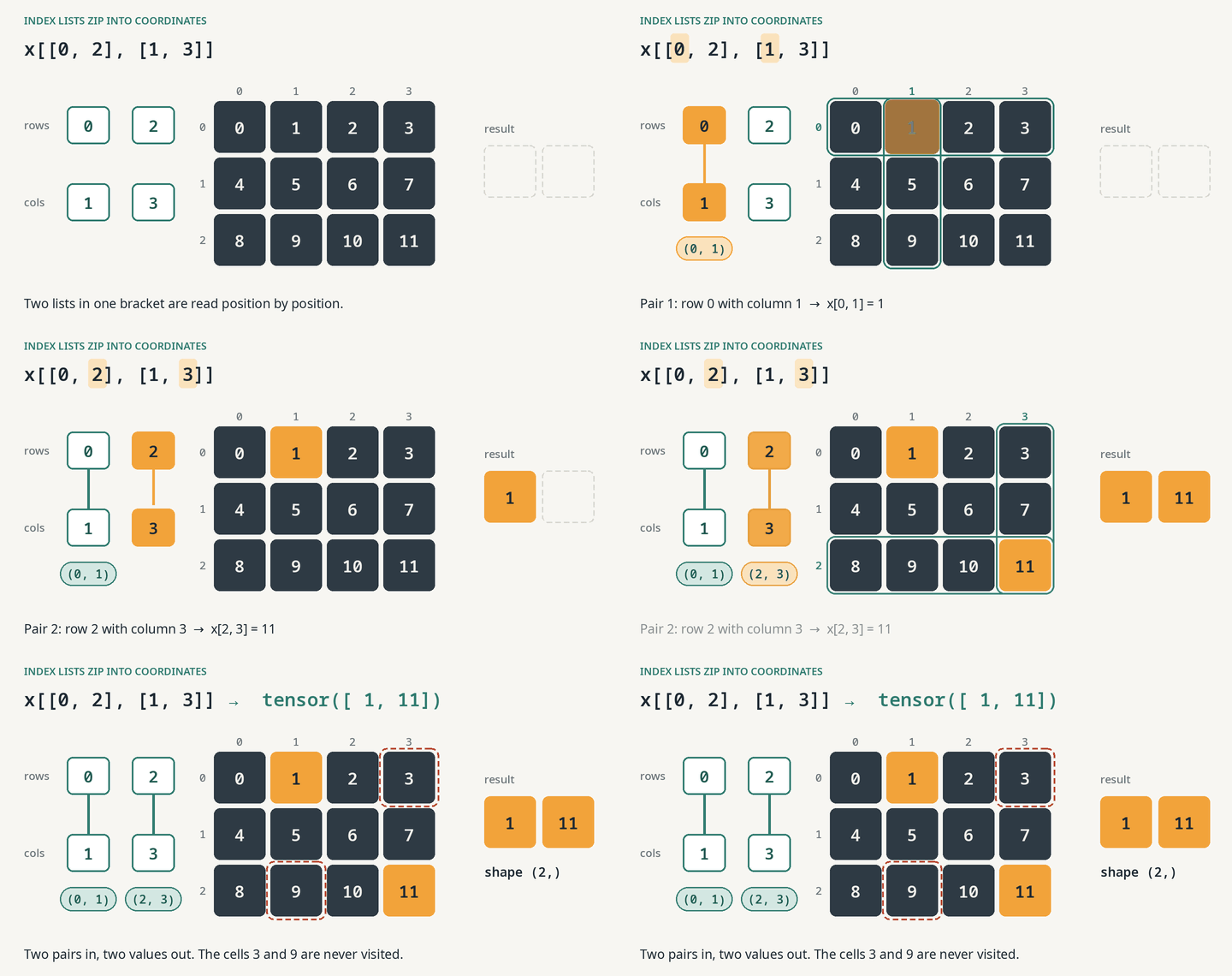
Now the first surprise. Give PyTorch a list of rows and a list of columns, and it does not take every combination. It pairs them like the two sides of a zipper: the first row with the first column, the second row with the second column, and so on. Each pair is the address of one cell, its coordinates, and each address yields one number. Rows 0 and 2 zipped with columns 1 and 3 give the cells (0, 1) and (2, 3): two numbers, 1 and 11, not four.
To get every combination, the two lists must be arranged so that they stretch into a grid, one standing as a column and the other lying as a row, using the broadcasting of stop 2.
The precise rule
Broadcast all the index tensors in the bracket to one shape. Every position in that shape is one coordinate, assembled from the matching entries of each index. The result has exactly that shape, with one value per coordinate.
For engineers
>>> x[[0, 2], [1, 3]]          # coordinates (0, 1) and (2, 3)
tensor([ 1, 11])
The zipper is a special case of a more general rule. All the index tensors in one bracket are first broadcast against each other, exactly as in stop 2, and the broadcast shape becomes the shape of the result. Two lists of shape (2,) broadcast to (2,): two coordinates, two values. To get the grid, we give the indexes shapes that broadcast to a grid, a column of row numbers and a row of column numbers:
>>> x[torch.tensor([[0], [2]]), torch.tensor([1, 3])]  # (2, 1) by (2,)
tensor([[ 1,  3],
[ 9, 11]])In plain English
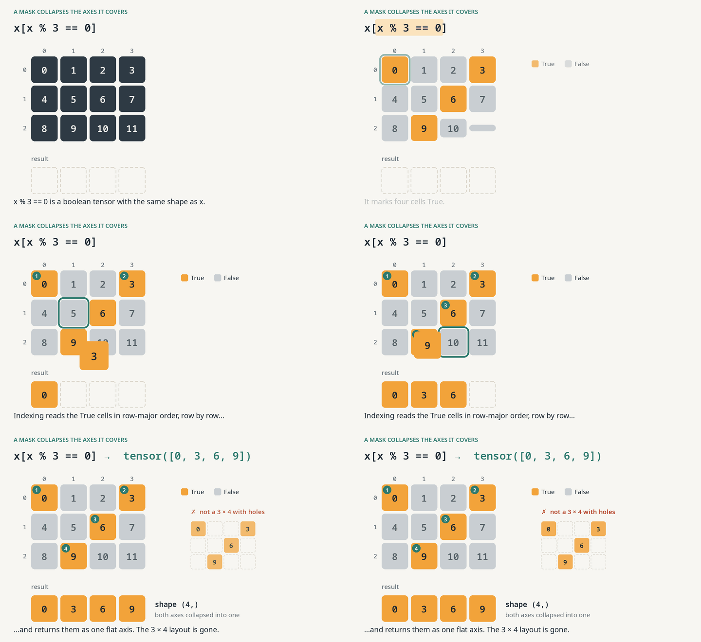
A mask is a grid of yes/no answers that marks the cells to pick, like a highlighter. When you index with a mask, PyTorch reads the highlighted cells in order, row by row, and returns them as a single flat line. The grid’s layout is gone: you get the selected values, not a picture of the original with gaps.
The order matters. PyTorch reads the highlighted cells the way you read a page: left to right along the first row, then the second, and so on. Turn the grid on its side and the same cells come out in a different order, because the rows are different.
The precise rule
A boolean mask in a slot is replaced by the coordinates of its True entries, listed in row-major order: row 0 from left to right, then row 1, and so on. A mask with k dimensions consumes k axes of the tensor and contributes a single axis whose length is the number of True values. The layout is not preserved, because the result is a list of selected elements, not a picture of the original.
For engineers
>>> x[x % 3 == 0]        # flat: the layout is gone
tensor([0, 3, 6, 9])
>>> x.T[x.T % 3 == 0]    # read in x.T's own row order
tensor([0, 9, 6, 3])
Row-major order is a property of the tensor being read, not of the values. Transpose it and the same four numbers come out in a different order, because x.T has four rows of three and is read row by row like everything else.
A mask does not have to cover every axis. A two-dimensional mask over the first two axes of t collapses those two axes into one and leaves the last axis alone:
>>> layrow = torch.tensor([[True, False, True], [False, True, False]])
>>> t[layrow].shape        # 3 trues, each picks a whole row of 4
torch.Size([3, 4])
>>> diag = torch.zeros(3, 4, dtype=torch.bool)
>>> diag[0, 0] = diag[1, 1] = diag[2, 2] = True
>>> t[:, diag].shape       # 3 trues, one per layer
torch.Size([2, 3])
Why it matters
The length of a masked result depends on the data, and that has two consequences. On a GPU, PyTorch has to count the True values before it can allocate the output, so x[mask] makes the host wait for the device, a synchronisation that can quietly serialise an otherwise asynchronous training step. And because the layout is gone, masking is the wrong tool whenever the shape must survive, for example when ignoring padded tokens in a batch. There the right call is torch.where, which keeps every position and changes only the values:
>>> torch.where(x % 3 == 0, x, torch.tensor(-1))
tensor([[ 0, -1, -1,  3],
        [-1, -1,  6, -1],
[-1, 9, -1, 11]]) # shape preservedIn plain English
A mask in a slot turns into the positions of its True values, so a one-dimensional mask becomes a single list of positions. From then on it behaves exactly like the lists of stop 4: it zips with other index tensors, broadcasts against integers, and leaves slices alone.
This is where intuition imported from other tools does the most damage. In a spreadsheet or a data table, selecting “these rows and these columns” usually means every combination: the Cartesian product. PyTorch does not do that. Two masks in one bracket are two lists of positions, and lists zip. They never multiply.
The precise rule
Two masks in one bracket are two position lists, and position lists zip. They never form a Cartesian product. If the True counts differ, the lists cannot broadcast and PyTorch raises an error; if the counts happen to match, it returns paired values without complaint.
For engineers
>>> x[rmask, cmask]      # two masks: zip, not grid
tensor([ 1, 11])
>>> x[rmask][:, cmask]   # chain: grid
tensor([[ 1,  3],
        [ 9, 11]])
Why it matters
In pandas, df.loc[row_mask, col_mask] selects every kept row crossed with every kept column: the Cartesian product. The same-looking expression in PyTorch, and in NumPy, pairs the masks entry by entry. When the counts differ we at least get an error. When they match, as in our example, we get a plausible-looking vector of the wrong values. To mean “these rows and these columns”, say so explicitly: chain the masks when reading, or build a grid of positions with [:, None] when writing, as in stop 8.
In plain English
A chain such as t[:, 1][0] is two separate indexing operations. The first produces a new tensor with its own directions, numbered from 0, and the second bracket indexes that tensor knowing nothing about where its directions came from. A single bracket, by contrast, addresses the original directions all at once. The same characters can therefore land on different directions.
For reading, a chain is legitimate and often the clearest way to say “these rows, then these columns”. For writing, everything depends on what the first bracket returns. A chain of basic indexes is windows all the way down, so a write at the end of it reaches the original.
![Animation on the two-layer tensor t: t[:, 1] removes the row direction, so the next [0] lands on the layer direction and returns [4, 5, 6, 7]; in one bracket t[:, 1, 0] keeps the original numbering and the 0 lands on the column direction, returning [4, 16].](/blog/media/kf9TjVzkovf4/gif_chained_axes.gif)
The precise rule
After each bracket, renumber the axes of the result from 0, then apply the next bracket to that. Every integer removes an axis, so the axes to its right shift one place left; every None inserts one, shifting the axes after it one place right.
For engineers
>>> t[:, 1][0]     # chain: first bracket drops rows, so [0] hits layers
tensor([4, 5, 6, 7])
>>> t[:, 1, 0]     # one bracket: 0 hits the column axis
tensor([ 4, 16])
Renumbering also explains the third surprise from the other side. Chaining two masks applies them one after the other, rows first and then the columns of that result, which is how we get the grid that a single bracket refuses to build.
For writing, everything depends on what the first bracket returns. A chain of basic indexes is views all the way down, so a write at the end of it reaches the original:
>>> x[1][0] = 99        # chain of basic indexes: write reaches x
>>> x[1, 0]
tensor(99)
Why it matters
A classic refactoring bug is collapsing a[:, i][j] into a[:, i, j] because it looks tidier. The two agree only when the first bracket contains nothing but integers. Chains also cost something at runtime: every bracket is a separate operation, and if one of them is advanced it allocates a full intermediate copy.
In plain English
Every indexing form we have met can also appear on the left of an assignment, and the core rule is refreshingly simple. x[idx] = v is a single call that writes into the memory of x itself, whatever kind of index idx is. Masks, lists and index tensors all write in place, and the value broadcasts to the shape of x[idx] under the one-way rule from stop 2.
The traps come from statements that look like one write but are not. There are two of them.
The chained write that goes nowhere
Python evaluates x[rmask][:, cmask] = 0 as x.__getitem__(rmask).__setitem__((slice(None), cmask), 0). The getitem builds a copy (stop 3), the setitem dutifully writes zeros into that copy, and the copy, referenced by nothing, is thrown away:
>>> x[rmask][:, cmask] = 0      # no error, no warning
>>> x
tensor([[ 0,  1,  2,  3],
        [ 4,  5,  6,  7],
        [ 8,  9, 10, 11]])
The fix is to put the whole selection into one bracket, so that the only call is a setitem on x. Two masks would zip (stop 6), so we either convert them to position lists shaped into a grid (stop 4) or combine them into one two-dimensional mask:
>>> x[rmask.nonzero().squeeze(1)[:,None], cmask.nonzero().squeeze(1)[None,:]] = 0
>>> x
tensor([[ 0,  0,  2,  0],
        [ 4,  5,  6,  7],
        [ 8,  0, 10,  0]])
>>> x2 = torch.arange(12).reshape(3, 4)
>>> x2[rmask[:, None] & cmask[None, :]] = 0   # one 2-D mask
>>> torch.equal(x, x2)
Truex writes into x itself.b[idx] += 1 expands to three steps: read b[idx], which gathers a copy; add 1 to the copy; and write the copy back with b[idx] = .... If idx repeats a position, the increments never accumulate. index_put_ with accumulate=True, or its siblings index_add_ and scatter_add_, adds every contribution:
>>> b = torch.zeros(3)
>>> b[torch.tensor([0, 0, 1])] += 1
>>> b
tensor([1., 1., 0.])
>>> b = torch.zeros(3)
>>> idx = torch.tensor([0, 0, 1])
>>> b.index_put_((idx,), torch.ones(3), accumulate=True)
tensor([2., 1., 0.])
Without accumulation, PyTorch’s documentation is explicit that writing to duplicate positions gives an undefined result. Our example only looks predictable because every write carries the same value.
Why it matters
Both traps produce results that look fine. Repeated positions are normal in real data: the same word appears twice in a sentence, many links point to the same page, many events land in the same bucket of a histogram. Counting them with += quietly undercounts. And the lost write turns up in exactly the code that must not fail silently: blanking out invalid entries, capping extreme values, resetting the state of a conversation that has finished.
Eight stops reduce to three sentences. Engineers can carry them in this compact form:
Indexes become coordinates, masks become true positions, position lists broadcast together.
In plain English:
Indexes become coordinates. Everything inside the brackets is an instruction for one direction of the grid, and together the instructions spell out addresses. Single numbers and ranges describe a regular pattern, so they give a window onto the original; anything that lists positions gives a photocopy. A new set of brackets means a new tensor, with its directions numbered afresh.
Masks become true positions. A highlighter is shorthand for the addresses of the highlighted (True) cells, read like lines on a page. That is why the multiples of three came back as a flat line, and why the grid turned on its side gave a different order.
Position lists broadcast together. All the lists of positions in one set of brackets are stretched to a common shape and read in step, one address per position: the zipper. That is why two lists gave two numbers, why two masks gave pairs, and why arranging the lists as a column and a row produces a grid.
The fourth surprise needs one more fact, about Python rather than PyTorch: an assignment writes into whatever the final brackets are attached to. If an earlier step made a photocopy, that is where the write goes, and it is thrown away with the copy.
| What goes in the brackets | Example | What happens to the shape | Window or photocopy? |
|---|---|---|---|
| A single number | x[1] | That direction disappears | Window (view) |
| A range (slice) | x[1:2] | That direction stays, perhaps shorter | Window (view) |
| None | x[:, None] | A new direction of size 1 appears | Window (view) |
| Ellipsis | y[0, ..., None] | Stands in for every direction not mentioned | Window (view) |
| A list of positions | x[[0, 2], [1, 3]] | The lists pair up (zip) and the result takes their combined shape, which moves to the front if a range separates them | Photocopy (copy) |
| A mask (highlighter) | x[x % 3 == 0] | The highlighted directions collapse into one line of the selected values | Photocopy (copy) |
rows[:, None] and cols[None, :].torch.where(mask, x, fill), which blanks cells instead of removing them.index_put_(..., accumulate=True), index_add_ or scatter_add_ so that every update counts..clone(), or the whole original stays in memory.None of this requires memorising special cases. It requires reading brackets the way PyTorch reads them: one direction at a time, one list of positions at a time, one result at a time. Once that habit forms, the four answers at the top of this page stop looking like surprises and start looking like the only possible answers. And the next time a recommendation lands just right or a translation reads naturally, it is worth remembering how much of that depended on picking exactly the right numbers.
| Word | Meaning |
|---|---|
| Tensor | A grid of numbers with any number of directions: a list, a table, or a stack of tables. |
| Axis (dimension) | One direction in a tensor, such as down the rows or across the columns. |
| Shape | The size of a tensor along each axis: 3 rows and 4 columns is shape (3, 4). |
| Index | A position number, counted from 0. Indexing means picking the values at chosen positions. |
| Slice | A range of positions, such as 1:3 for positions 1 and 2. |
| Mask | A grid of True/False answers that marks the cells to pick, like a highlighter. |
| Broadcasting | Stretching a direction of size 1 so that two shapes fit together. |
| View | A window onto the original data. Changes made through it change the original. |
| Copy | A photocopy of the selected data. Changes made to it stay in the copy. |
| In place | Changing the original tensor rather than producing a new one. |
| GPU | The specialised chip that runs most AI computation. |

Thoughts and essays, published with Yokush. See more posts
 Siddharth14 min
 Siddharth19 min2
Comments 0