The 96% Solution: How to Cut LLM Costs by 96% in 90 Days — Without Sacrificing Quality

Siddharth
June 13, 202613 min read

A vendor-agnostic playbook for engineering and finance leaders, built on three layers of compounding optimization. Every number comes from production workloads. Every lever is something you can deploy on Monday.
Most enterprises are running production LLM workloads at 2–10× the cost they should be paying. Not because the models are too expensive — list rates for a representative frontier call run $2–5 per million input tokens and $12–25 per million output tokens. The waste lives in how the calls are made, what context they carry, and which model they use.
Cloud FinOps frameworks do not transfer cleanly to AI workloads. An LLM call has no taggable resource at the point of use, costs vary by an order of magnitude across consecutive requests, and a single prompt change can 10× the bill overnight. Treating this as a procurement problem — negotiating enterprise discounts, comparing list prices — addresses roughly 5% of the actual surface area. The remaining 95% is an application-layer problem: it lives in how you write prompts, choose models, structure context, and orchestrate calls.
Cost per million tokens is an engineering metric. Cost per resolved ticket, per analyst-hour saved, per draft generated — these are the numbers the business will fund.
The good news: the savings stack multiplicatively, not additively. A workload running on a mid-tier model with 70% cache hit rate and async batch processing moves from $3 / $15 per million tokens to roughly $0.60 / $3.75 — an 80% reduction with no quality change. Stack the architectural patterns on top, and the same workload lands at 3–6% of naive baseline at the same evaluation acceptance. That is not a procurement outcome. It is a discipline outcome.
Most teams instrument two of the seven billable components in an LLM call and miss the rest. Here is the full anatomy of what shows up on a monthly invoice:
| Component | What it is | Typical cost vs base input |
|---|---|---|
| Standard input | Prompt + system + tools + history | 1.0× |
| Cached input | Repeated prefix served from provider cache | 0.1× (90% off) |
| Cache write | First-time write of a cached block | 1.25× / 2.0× |
| Output | Visible response tokens | 4–6× input |
| Reasoning (hidden) | Internal chain-of-thought, billed as output | 5–20× visible output |
| Tool / search | Web search, file search, code execution, grounding | $25–$35 per 1k calls |
| Storage & sidecars | Vector DB, embeddings, cache-storage hours, observability | Provider-specific |
The line items most enterprises miss are the ones that quietly compound. Reasoning tokens on o-series and extended-thinking modes are invisible to the user but bill at the output rate — a 1K visible answer can easily generate 10K+ reasoning tokens, multiplying effective output cost by an order of magnitude. Long-context cliffs charge 2× input and 1.5× output above provider-specific thresholds (200K tokens for one major vendor, 272K for another), with no visible warning until the bill arrives. Tool fees per 1K grounding searches can exceed the token cost of the call itself. And cache storage hours on a 100K-token cache held for 24 hours run ~$10/day — a real number once caches accumulate.
The single largest source of waste, however, is the one most teams accept as inevitable: using a frontier model where a mid-tier or cheap model would do. Routing typically captures 40–70% of available savings before any other lever is touched. Output discipline, the second-largest lever, is nearly free: a 30% reduction in average output tokens cuts the bill 20–25% on an output-heavy workload, and structured outputs typically drop output tokens 40–60%.
The reason a properly executed AI cost program lands at 96% reduction rather than 60% is that the savings compound. Each layer of the cascade is built on the prior layer's reduced baseline. The playbook documents the effect in three explicit stages: the twelve operational levers deliver ~88% reduction, the six foundational patterns add another 40–55% on the post-lever remainder to land at ~94% off the naive bill, and the six advanced approaches push the final figure to 3–6% of baseline at the same evaluation acceptance. The waterfall below traces a representative mid-complexity workload (50M tokens/day, 70% input share) through eight stages:
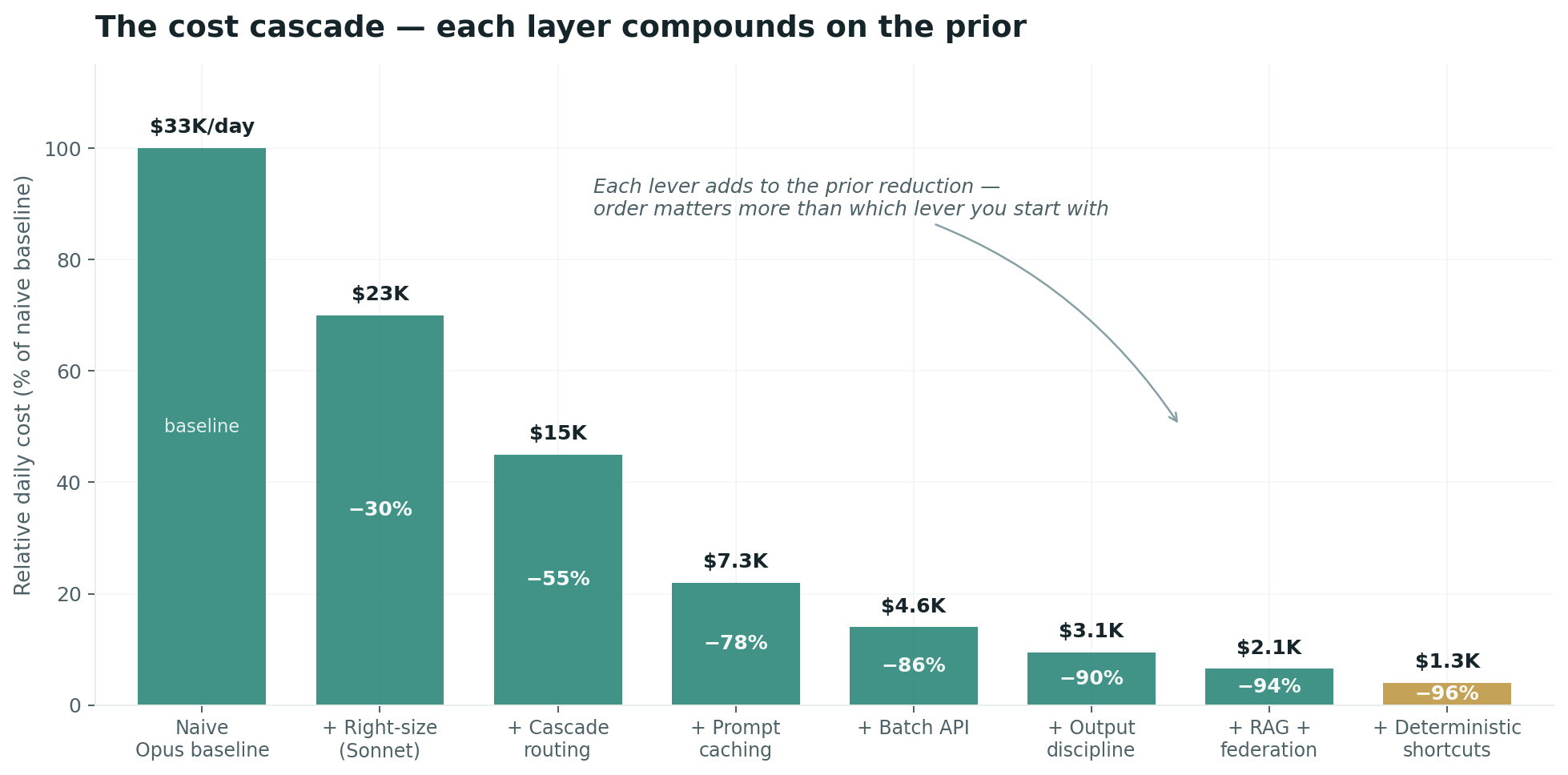
The order is the insight. Naive cost discipline attacks one lever hard — usually batching or compression — and reports a 30% win. Disciplined cost programs sequence the levers so each one's savings carry forward to the next baseline. By the time you reach the architectural patterns, you are not optimizing a 100% bill; you are optimizing the 12% that survived the lever cascade. That is where the most surprising gains appear.
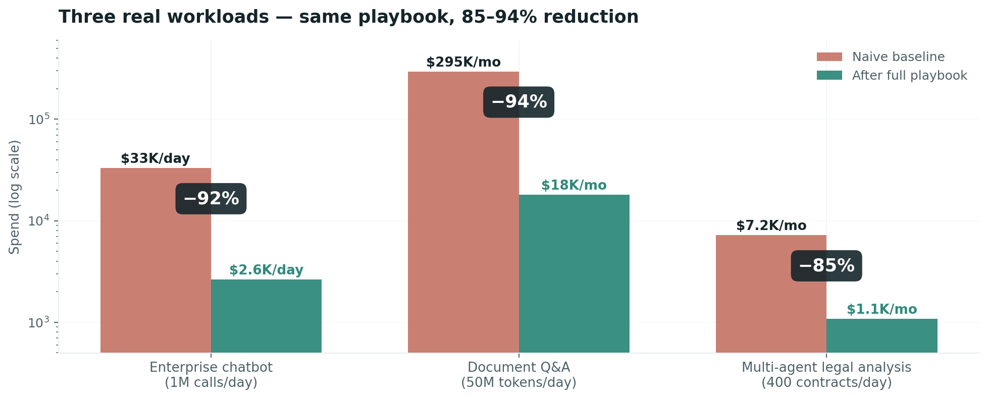
The three examples above are not edge cases. They are the playbook's published workload transformations: a high-volume customer-facing chatbot, a knowledge-base question-answering system, and a multi-step agent doing structured work on documents. All three hit 85%+ reduction. The Document Q&A case is the most instructive — RAG alone captures 78% of the savings, because the workload's bottleneck was always context length, not model intelligence. Replacing 200K-token context stuffing with retrieved 1K-token chunks solves the cost problem and improves latency as a side effect.
If you do nothing else from this playbook, do these three things. Each is implementable in a single sprint. None requires an architectural redesign. Together they capture the majority of the available savings, and everything else is incremental on top.
max_tokens on every callOutput tokens are 4–6× input. The default provider behavior is to generate until the model decides to stop, which for reasoning models can run into the thousands. For the vast majority of production calls — classification, extraction, format conversion, summarization — the answer fits in 200–800 tokens. Setting a per-feature max_tokens cap is a five-line code change. It costs nothing to enable. It prevents entire classes of overrun. It is the single highest-ROI intervention in the entire cost program, and most production codebases are missing it.
The pattern: enforce a per-feature max_tokens policy in the gateway, refuse calls without it, and set the hard ceiling above your expected p99 plus a buffer. For interactive chat, 600–1,500 is usually correct. For classification, 200 is plenty. For long-form drafting, 4,000 is the upper bound before you should be using a specialized workflow.
Provider prompt caches charge 10% of base input cost for cached tokens. Cache writes are 1.25× (5-minute TTL) or 2× (1-hour TTL) of base. The break-even is fast: one read for 5-minute TTL, two reads for 1-hour. For RAG and agentic workloads with a stable system prompt and tool definitions, this is a free 70–90% input cost reduction.
The implementation is mechanical. Place stable content — system prompt, tool definitions, retrieved documents, few-shot examples — at the top of the prompt. Mark cache breakpoints in the API call. Use 5-minute TTL by default and switch to 1-hour only if call patterns are sparse. Track cache hit rate per route; the target is 70% or higher on any cacheable workload. On a 1M-call-per-day mid-tier workload with a 5K-token stable prefix, a 70% hit rate recovers $1,500–$2,000 per day. Per day.
The most expensive mistake in production AI is running a cheap task on a frontier model. The fix is not a feeling — it is a calibration matrix. Build a 50-case held-out eval set per task class. Run it against the cheap, mid-tier, and frontier model. Pick the cheapest model that hits your acceptance threshold (typically 95% of the best model's quality). The cost difference is 5–25× on input, 5–10× on output.
A representative run — 50 cases × 6 task classes × 6–10 candidate models — costs $20–50 in API calls and 30 minutes of compute. The matrix it produces drives millions of subsequent routing decisions. It is the highest-leverage spend in the entire program. Re-run it quarterly. Re-run it every time a major model version lands.
Once the three big levers are in production, the work moves from configuration to architecture. The patterns below are not optional once token volume crosses ~50M tokens/day, the agent has more than a handful of tools, or conversations stretch beyond ten turns. They are the difference between a cost program that plateaus at 70% and one that lands at 96%.
Every routing decision in your system should trace back to a calibration matrix. A calibration matrix is a reproducible score of every (task class × model) pair on quality, cost, latency, and hallucination rate. The acceptance rule: pick the cheapest model where quality is at least 95% of the best model on that class. This is the artifact that makes "right-sized routing" empirical rather than tribal. Without it, you are guessing.
Different providers win different task classes. One vendor's cheap tier may be your best quality-to-cost option for classification; another vendor's mid-tier may dominate for code generation. The calibration matrix tells you who wins where. A gateway enforces the routing and handles failover. On a 50M token/day workload spread across five task classes, optimal cross-provider routing typically beats the best single-provider strategy by 15–25% at the same eval acceptance. Failover is a free bonus — when one provider has a regional incident, your traffic reroutes automatically.
The default of sending everything that might matter is what bleeds the bill. Treat context as a federated set of segments: system prompt, tool definitions, retrieved documents, persona, history, skill instructions, knowledge cards. Each segment has an ID, a relevance scorer, a token budget, and a lazy loader. Per call, the orchestrator decides which segments to load based on the current query, fills a global token budget in priority order, and stops. A typical agent call sends 25–40K tokens of context, of which 60–75% is irrelevant to the current turn. Federation reduces that to the relevant 8–12K. On a 1M-call-per-day mid-tier workload, that is $1,500–$2,500 per day recovered.
Don't ship every tool definition on every call. Forty tools at 200 tokens each is 8K tokens of definitions per call — about $24,000 per day on a 1M-call mid-tier workload. The federated approach: stage one is a vector recall to 15 candidate tools, stage two is a cheap-model call that returns the 3–5 most likely-relevant tool IDs, stage three is the main call with only those definitions injected. Discovery cost is roughly $0.0003 per call. The savings on 40→5 tools, at 1M calls per day, is roughly $19,000 per day. Track discovery accuracy; the target is that the agent needed a tool that wasn't discovered in less than 1% of calls.
Visibility alone does not prevent runaways — controls do. The architecture is layered so that no single failure (a buggy retry loop, a leaked API key, a runaway agent) can spend more than its blast radius.
Preventive controls run on every call and cost nothing to enable: per-feature model whitelists, max_tokens caps, hard token-budget per request. They prevent entire classes of overrun. The gateway enforces them; no application can opt out.
Detective controls monitor spend velocity, not cumulative spend. A workload that is going to overrun does so by accelerating — the alert needs to fire before the overrun, not after. The four core signals: 5-minute burn rate against per-feature daily budget (alert at 1.5×), cache hit rate floor (alert on regression below 50% for any cacheable feature), reasoning-token share (alert above 20% on non-reasoning features), and tier-mix drift (alert if a route's mid-or-frontier share exceeds expected by more than 15 percentage points).
Corrective controls are behaviors, not Slack messages. When the alert fires, the system acts. Tier-down: automatically route incoming traffic from frontier to mid, or mid to cheap, with a user-visible quality flag. Queue and degrade: redirect non-interactive calls to the async batch tier (24-hour SLA, 50% off). Hard kill-switch: per-feature token-spend cap that 429s the feature when exceeded, with a clean error path. The blast radius is the feature, not the platform.
All three layers should live behind an AI gateway — a single proxy in front of every LLM call that centralizes keys, budgets, model whitelists, fallbacks, and instrumentation. Centralizing policy in one place, not in every application, is the difference between controls that hold and controls that decay. Every team integrating against the gateway inherits the limits, alerts, and breakers automatically.
Built for a team starting from no instrumentation, no controls, and no allocation — which is most enterprise AI today. Each phase lands a working capability. Nothing is left for "phase four."
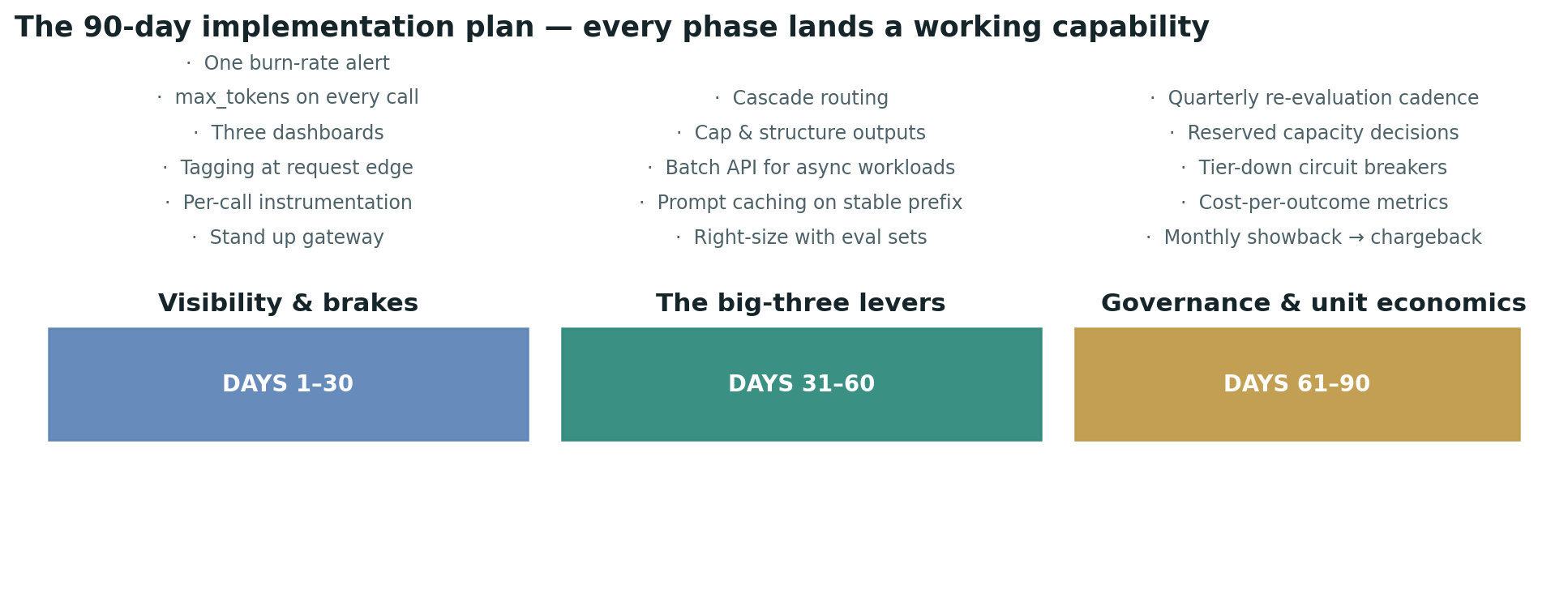
Days 1–30 — Visibility and brakes. Stand up a gateway in front of all LLM traffic. Instrument per-call usage records. Tag every call at the request edge with tenant, feature, and cost center. Deploy three dashboards. Enable max_tokens on every call. Wire one alert — spend velocity above 1.5× daily target. Inventory your current LLM workloads. This is your optimization backlog.
Days 31–60 — The big-three levers. Build per-feature eval sets and run the calibration. Move every feature to the cheapest tier that passes acceptance. Enable prompt caching on every workload with a stable prefix; reorganize prompts so cacheable content is contiguous and at the top. Move batchable workloads to the async batch tier. Cap and structure outputs. Deploy cascade routing on heterogeneous workloads. Expect 40–60% blended savings from this phase alone.
Days 61–90 — Governance and unit economics. Stand up monthly showback to product and business-unit leads. Define cost-per-outcome metrics: dollars per ticket resolved, per draft generated, per analysis completed. Add the corrective layer — tier-down circuit breakers, per-feature kill-switches, queue-and-degrade for batchable overflow. Decide on reserved-capacity commitments for the top three highest-volume workloads. Establish the quarterly model-evaluation cadence. Document the RACI and put each role on a named owner. Without named ownership, this whole apparatus decays.
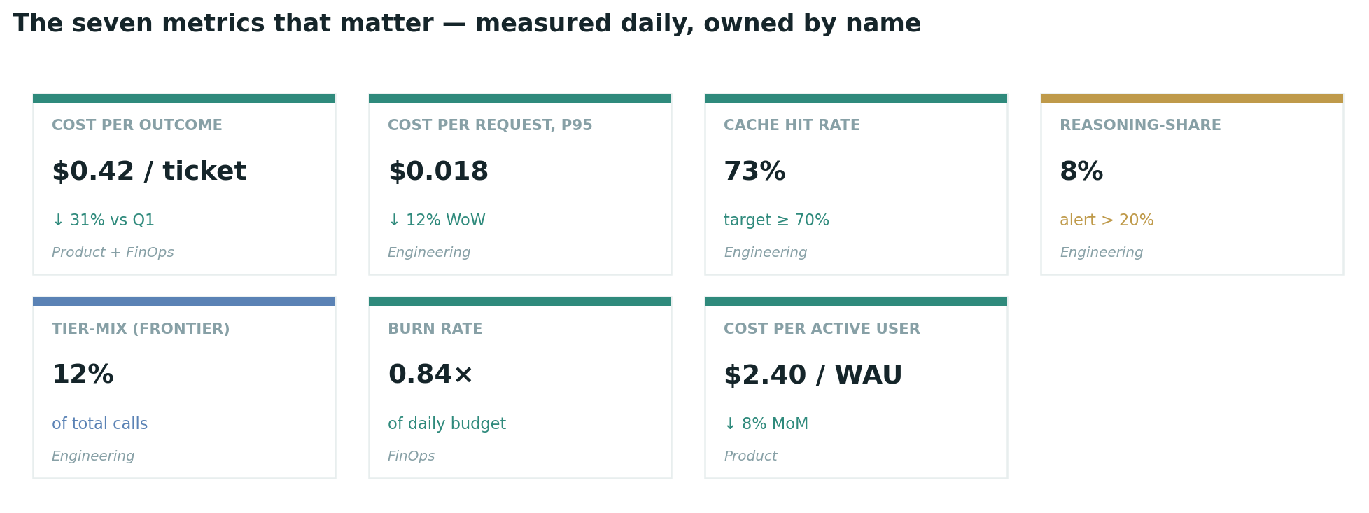
The single most common failure mode in AI cost programs is reporting the wrong number. Cost per million tokens is an engineering metric. It is accurate, it is precise, and it is irrelevant to the CFO. The numbers that fund programs and survive CFO scrutiny are outcome-based:
| Metric | Definition | Cadence | Owner |
|---|---|---|---|
| Cost per outcome | $ per resolved ticket / drafted memo / closed task | Daily | Product + FinOps |
| Cost per active user | Total AI spend ÷ WAU | Weekly | Product |
| Cost per request, p50 / p95 | Distribution of $ per API call, by route | Daily | Engineering |
| Cache hit rate | Cached input tokens ÷ total input tokens, by route | Hourly | Engineering |
| Reasoning-share | Reasoning tokens ÷ total output tokens, by route | Hourly | Engineering |
| Tier-mix | % of calls by model tier (frontier / mid / cheap) | Daily | Engineering |
| Burn rate | $ spent today ÷ daily budget; alert at 1.5× | 5-minute | FinOps |
The first metric — cost per outcome — is the one to lead with. It is the metric that translates AI spend into business value, that aligns engineering incentives with product outcomes, and that survives a finance review. The other six are diagnostic. They tell you why cost per outcome moved. They do not justify the program on their own.
If you remember nothing else, remember this: the three highest-leverage interventions in AI cost discipline are max_tokens on every call, prompt caching on the stable prefix, and right-sizing the model with an eval set. These three changes, in 4 weeks of focused work, typically capture 70–80% of the available savings. Everything else in this playbook is incremental on top. Start there. Measure the impact. Then move to architectural patterns.
The mistake to avoid is treating AI cost as either a cloud problem or a model-procurement problem. It is neither. It is an application-layer problem — the costs are generated by how you write prompts, choose models, structure context, and orchestrate calls. The financial discipline has to live where the engineering decisions are made.
Providers and prices will move. Provider-specific features will land and retire. New model tiers will appear. The structure — measure, control, optimize, with clear unit economics and named ownership — outlasts any specific generation of models. The teams that get this right do not build AI cheaply by accident. They build it cheaply because every decision — model, prompt, context, output, route — is made with cost as a first-class design constraint, not a quarterly invoice surprise.
Thoughts and essays, published with Yokush. See more posts
 Siddharth21 min
 Siddharth24 min11
 Siddharth11 min
Comments 0