Three independent engineering breakthroughs—NVFP4 quantization compressing model memory by 75%, Long RoPE extending context windows 32–256× beyond training length, and Multi-Token Prediction enabling parallel token generation—compound to multiply inference throughput 3–10× on existing hardware. The key takeaway: these techniques stack multiplicatively, not additively, meaning a single GPU can now serve 3× more concurrent users while processing entire documents in one pass, fundamentally rewriting the economics of LLM deployment without requiring new silicon.
Three distinct engineering breakthroughs — one compressing the weights, one extending the reach, one multiplying the output — are converging to make every inference dollar go dramatically further. Here's how they work, why they compound, and what they mean for your infrastructure bill.
Large language models generate text one token at a time. That sounds simple, but the mechanics are brutal: each new token requires the GPU to load the entire model — every weight, every layer, plus a growing key-value cache — from VRAM into the compute cores, run a full forward pass, produce a single token, and repeat. On a 70-billion-parameter model, that's roughly 140 gigabytes of data movement per token.
This is why inference is memory-bandwidth bound, not compute-bound. Your GPU's tensor cores sit idle most of the time, waiting for data to arrive. The teraflops on the spec sheet are irrelevant if the memory highway can't feed them fast enough.
Three independent innovations attack this bottleneck from different angles. None requires new silicon you don't already own. Stacked together, they don't add — they multiply.
Let's break down each layer for both the engineer who needs to implement it and the executive who needs to justify the budget.
NVFP4 is a 4-bit floating-point quantization format introduced with the Blackwell GPU architecture. Each value is stored in an E2M1 layout — 1 sign bit, 2 exponent bits, 1 mantissa bit — yielding just 16 representable codes spanning approximately −6 to +6.
The genius is not in the 4 bits. It's in the two-level micro-block scaling layered on top:
Fig 1 — NVFP4 two-level scaling: 16 elements per block, each sharing an FP8 (E4M3) inner scale, with an optional FP32 outer scale across the tensor.
What distinguishes NVFP4 from the earlier MXFP4 format is the combination of smaller blocks (16 elements vs 32) and a richer scale type (FP8 E4M3 with 256 distinct values vs MXFP4's power-of-2 E8M0 with only magnitude steps). The FP8 scale is a real floating-point number, not just a power of two — so weights that fall between MXFP4's grid points survive quantization intact . The optional FP32 outer scale handles multi-magnitude activation outliers without contaminating every local block's precision.
The results, per NVIDIA's benchmarks and independent evaluations: roughly 4× memory reduction vs FP16/BF16, 1.5–1.8× smaller than FP8, with accuracy loss typically under 1% — and accuracy recovery improves with model size, making NVFP4 strongest on large dense and mixture-of-experts architectures .
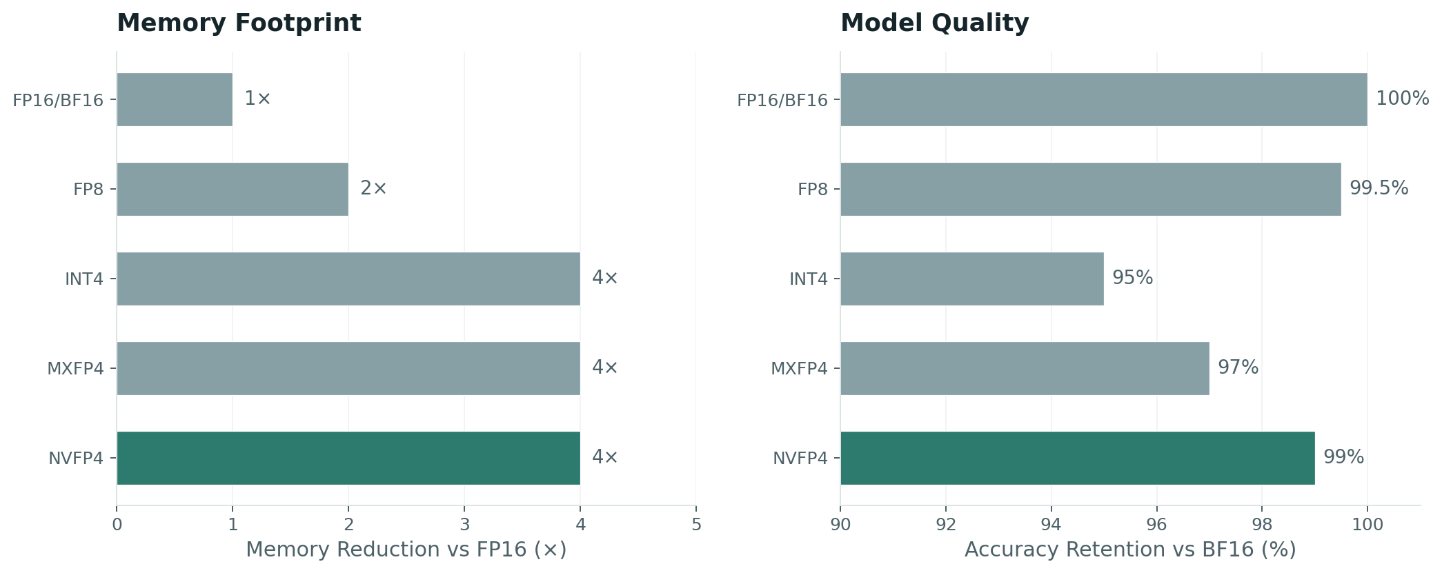
Think of NVFP4 as compressing your model's memory footprint by 75% while keeping almost all its intelligence intact.
A typical 70-billion-parameter model in 16-bit precision occupies about 140 GB of VRAM. In NVFP4, that drops to roughly 35 GB. On a single GPU with 96 GB of VRAM, you go from not fitting at all to fitting with room for multiple concurrent users. The implications compound:
Concrete example: A customer-service chatbot running a 32B model on a single GPU. In FP16, the model fills most of the VRAM, leaving room for perhaps 4–6 concurrent conversations. Switch to NVFP4, and the freed memory allows 12–16 concurrent conversations on the same hardware — a 3× capacity increase with zero additional spend and under 1% quality loss.
Rotary Position Embedding (RoPE) is how virtually every modern LLM encodes token order. Instead of adding a position vector to each token's embedding, RoPE rotates the query and key vectors by an angle proportional to the token's position in the sequence . The elegant property: the attention dot product between positions m and n depends only on their relative distance m − n, not their absolute position
.
Fig 3 — RoPE encodes position as rotation. The problem: beyond the training boundary, rotation angles are unexplored territory.
The problem emerges when you feed the model a sequence longer than it was trained on. Positions beyond the training length produce rotation angles the model has never encountered. Attention distributions shift, softmax entropy changes, and the model starts "forgetting" information — especially in retrieval tasks where a key fact sits 100,000 tokens back.
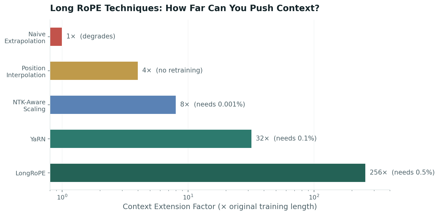
"Long RoPE" is the family of techniques that fix this without retraining from scratch:
| Technique | Mechanism | Trade-off |
|---|---|---|
| Position Interpolation | Compress position indices into trained range | Nearby-position resolution collapses |
| NTK-Aware Scaling | Rescale the base frequency to shift the frequency spectrum | High-frequency dims still lose resolution |
| YaRN | Hybrid interpolation + extrapolation with entropy correction | Needs ~0.1% continued pretraining (~400M tokens) |
| LongRoPE | Evolutionary search finds non-uniform per-dimension scaling | Compute-heavy tuning; model-specific |
Without position encoding, a language model treats "Alice loves Bob" and "Bob loves Alice" as identical — it has no concept of word order. RoPE is how the model knows what comes first, second, and thousandth.
But models are trained with a fixed "attention span" — typically 4,000 to 32,000 tokens. Feed them a 100,000-word document and they get confused about ordering because they've never encountered positions that far out. Long RoPE techniques teach the model to handle sequences far beyond its original training length, without expensive retraining.
Why this matters for your business:
Concrete example: A legal firm processing M&A due diligence. With a standard 8K context, a 120-page merger agreement must be split into ~15 chunks, each analyzed independently. Cross-references between page 3 and page 97 are invisible to any single chunk. With YaRN-extended context at 128K, the model reads the entire document in one pass. The due-diligence report catches an indemnification clause on page 12 that conflicts with a representation on page 89 — something no chunk-by-chunk approach would find.
Standard autoregressive generation is strictly sequential: each token requires a complete forward pass through the entire model. To produce 5 tokens, you need 5 sequential passes — and each pass is memory-bandwidth bound, meaning the GPU spends most of its time loading weights and waiting, not computing.
Multi-Token Prediction (MTP) converts this sequential problem into a parallel one using a two-pass speculation-and-verification scheme:
Fig 5 — MTP converts sequential generation into a two-pass speculate-verify pipeline. All guesses verified in a single parallel forward pass.
In the speculation pass, the model emits one confirmed token plus a block of guesses for the next k tokens. In the verification pass, it processes the entire sequence (prompt + confirmed token + guesses) in a single parallel forward pass and checks each guess against its own prediction. Guesses are accepted until the first mismatch.
The critical distinction from standard speculative decoding: traditional spec-dec requires loading a second, smaller draft model into VRAM alongside the main model. MTP uses built-in prediction heads trained into the same weights — zero additional memory. Reported speedups: approximately 2.5× for conversational text, up to 5× for predictable content like code, and over 3× on reasoning benchmarks per a February 2026 paper from University of Maryland and collaborators .
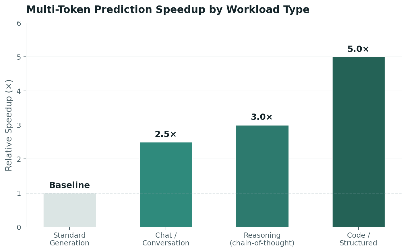
Right now, AI models generate text one word at a time, sequentially — like a typist who must finish each word before starting the next. MTP teaches the model to predict several words ahead, then verify them all at once — like composing a sentence in your head, then writing it down.
Instead of 5 separate computations for 5 words, the model does 2: one to predict, one to verify. The result is a 2.5–5× speedup depending on how predictable the content is.
Why this matters for your business:
Concrete example: A code-completion tool powered by a 34B model. Without MTP, generating a 50-line function takes roughly 8 seconds of sequential token generation — long enough that developers tab away. With MTP at 4× speedup for structured code, the same function appears in 2 seconds. The developer never leaves flow state. The tool goes from "occasionally useful" to "always on."
Here's where it gets interesting. These three techniques are orthogonal — they attack different bottlenecks. NVFP4 reduces how much data moves per pass. Long RoPE extends how many tokens the model can attend to. MTP reduces how many passes you need. Stacked together, the gains multiply, not add.
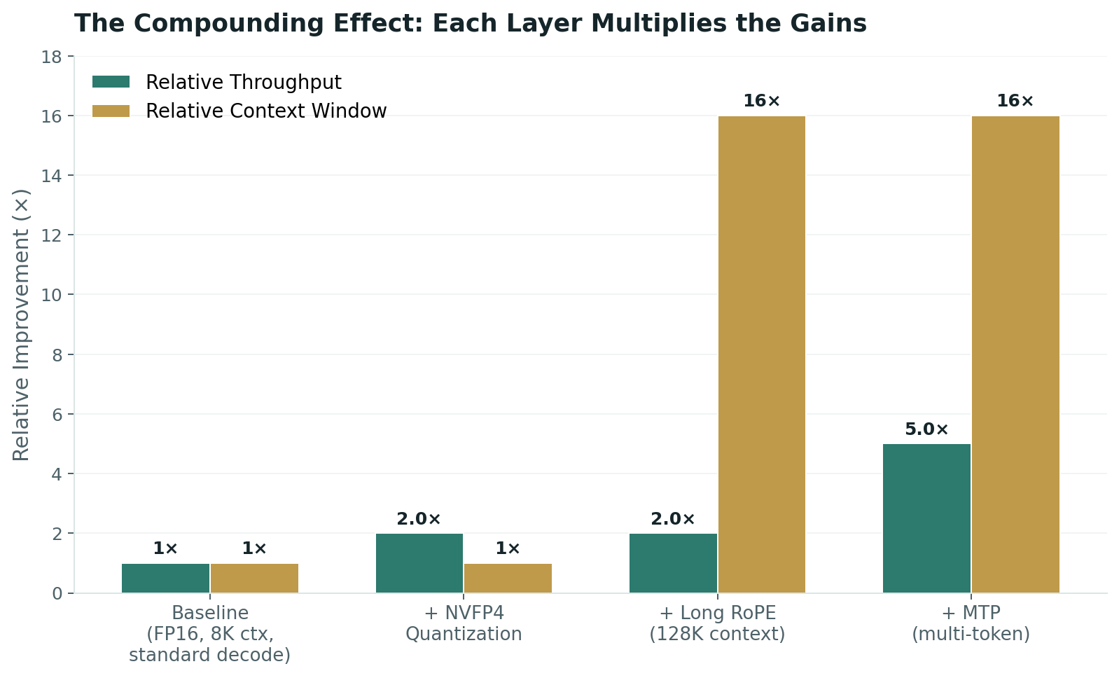
A model that previously required four GPUs, could only read 8,000 tokens, and generated 40 tokens per second becomes a model that fits on one GPU, reads 128,000 tokens, and generates 200 tokens per second — on the same silicon.
| Metric | Baseline (FP16, 8K, standard decode) | Optimized (NVFP4 + YaRN + MTP) | Improvement |
|---|---|---|---|
| Memory footprint (70B model) | ~140 GB | ~35 GB | 4× |
| Max context window | 8,000 tokens | 128,000+ tokens | 16× |
| Generation speed (code) | ~40 tok/s | ~200 tok/s | 5× |
| GPUs required | 2–4 | 1 | 75% reduction |
| Accuracy degradation | — | <1–2% | Negligible |
For the executive evaluating AI infrastructure spend, these three technologies collectively represent the difference between a deployment that requires a dedicated GPU cluster and one that runs efficiently on existing hardware. The economics are straightforward:
For the engineer, the implementation path is clear and each layer is independently deployable:
The next doubling of inference performance won't come from a new chip. It will come from stacking the three techniques that make the chips we already have work dramatically harder.
The companies that understand this stack — and implement it before their competitors do — will deliver AI experiences that are simultaneously faster, cheaper, and more capable. That's not a marginal optimization. That's a structural advantage.
Thoughts and essays, published with Yokush. See more posts


Comments 0